TOPIC: SAS
Cross-platform file and directory renaming in SAS with added return code handling
Here is another post on operating system-level actions performed from within SAS for the sake of being both robust and cross-platform. File deletion has been one example, so here is file and directory renaming. That got used while doing some debugging as well as a piece of validation testing.
The rename function applies to more than files, though, which means that the "FILE" parameter (in quotes below) is as essential as those for source and target file paths. That tripped me up when I went about doing it for the first time. All the action happens within a data step:
data _null_;
	rc = rename("&file_name..xlsx", "&file_name..bak", "FILE");
	if rc = 0 then
		putlog "File renamed successfully";
	else;
		putlog "Rename failed";
		msg = sysmsg();
		putlog "SYSMSG: " msg;
run;
Here, we have a null data step, which means that no output is written to disk. We also capture the return code for the operation in a variable called rc. If that has a value of 0, the operation has completed successfully, while the alternative can have extra information that can be captured by the sysmsg function, as is seen above. Putting this all together, not only can you issue the result of the operation in the log using putlog statements, but also extra information useful for debugging what happened and fixing it.
As has been alluded earlier, the rename function can be used with other objects too. Instead of "file", you can have these for those: "ACCESS" for an access descriptor that was created using SAS/ACCESS software, "CATALOG" for a SAS catalog or catalog entry, 'DATA' for a SAS table or dataset (which is the default and explains how I got caught out as mentioned earlier), "VIEW" for a SAS table view. That makes it more useful, even if the DATASETS procedure is worth checking out for some of these.
Some R packages to explore as you find your feet with the language
Here are some commonly used R packages and other tools that are pervasive, along with others that I have encountered while getting started with the language, itself becoming pervasive in my line of business. The collection grew organically as my explorations proceeded, and reflects what I was trying out during my acclimatisation.
General
Here are two general packages to get things started, with one of them being unavoidable in the R world. The other is more advanced, possibly offering more to package developers.
You cannot use R without knowing about this collection of packages. In many ways, they form a mini-language of their own, drawing some criticism from those who reckon that base R functionality covers a sufficient gamut anyway. Nevertheless, there is so much here that will get you going with data wrangling and visualisation that it is worth knowing what is possible. The complaints may come from your not needing to use anything else for these purposes.
This R package enables developers to convert existing R functions into web API endpoints by adding roxygen2-like comment annotations to their code. Once annotated, functions can handle HTTP GET and POST requests, accept query string or JSON parameters and return outputs such as plain values or rendered plots. The package is available on CRAN as a stable release, with a development version hosted on GitHub. For deployment, it integrates with DigitalOcean through a companion package called {plumberDeploy}, and also supports Posit Connect, PM2 and Docker as hosting options. Related projects in the same space include OpenCPU, which is designed for hosting R APIs in scientific research contexts, and the now-discontinued jug package, which took a more programmatic approach to API construction.
Data Preparation
You simply cannot avoid working with data during any analysis or reporting work. While there is a learning curve if you are used to other languages, there is little doubt that R is well-endowed when it comes to performing these tasks. Here are some packages that extend base R capabilities and might even add some extra user-friendliness along the way.
The {forcats} package in R provides functions to manage categorical variables by reordering factor levels, collapsing infrequent values and adjusting their sequence based on frequency or other variables. It includes tools such as reordering by another variable, grouping rare categories into 'other' and modifying level order manually, which are useful for data analysis and visualisation workflows. Designed as part of the tidyverse, it integrates with other packages to streamline tasks like counting and plotting categorical data, enhancing clarity and efficiency in handling factors within R.
Around this time last year, I remember completing a LinkedIn course on a set of good practices known as tidy data, where each variable occupies a column, each observation a row and each value a single cell. This package is designed to help users restructure data so it follows those rules. It provides tools for reshaping data between long and wide formats, handling nested lists, splitting or combining columns, managing missing values and layering or flattening grouped data.
Installation options include the {tidyverse} collection, standalone installation, or the development version from GitHub. The package succeeds earlier reshaping tools like {reshape2} and {reshape}, offering a focused approach to tidying data rather than general reshaping or aggregation.
Having a long track record of working with SAS, {haven} with its abilities to read and write data files from statistical software such as SAS, SPSS and Stata, leveraging the ReadStat library, arouses my interest. Handily, it supports a range of file formats, including SAS transport and data files, SPSS system and older portable files and Stata data files up to version 15, converting these into tibbles with enhanced printing capabilities. Value labels are preserved as a labelled class, allowing conversion to factors, while dates and times are transformed into standard R classes.
While there are other approaches to working with databases using R, {RMariaDB} provides a database interface and driver for MariaDB, designed to fully comply with the DBI specification and serve as a replacement for the older {RMySQL} package. It supports connecting to databases using configuration files, executing queries, reading and writing data tables and managing results in chunks. Installation options include binary packages from CRAN or development versions from GitHub, with additional dependencies such as MariaDB Connector/C or libmysqlclient required for Linux and macOS systems. Configuration is typically handled through a MariaDB-specific file, and the package includes acknowledgments for contributions from various developers and organisations.
For many people, the pandemic may be a fading memory, yet it offered its chances for learning R, not least because there was a use case with more than a hint of personal interest about it. Here is a library making it easier to get hold of the data, with some added pre-processing too. Memories of how I needed to wrangle what was published by various sources make me appreciate just how vital it is to have harmonised data for analysis work.
Table Production
While many appear to graphical presentation of results to their tabular display, R does have its options here too. In recent times, the options have improved, particularly of the pharmaverse initiative. Here is a selection of what I found during my explorations.
Part of the {officeverse} along with {officedown}, {Flextable}, {Rvg} and {mschart}, the {officer} R package enables users to create and modify Word and PowerPoint documents directly from R, allowing the insertion of images, tables and formatted content, as well as the import of document content into data frames. It supports the generation of RTF files and integrates with other packages for advanced features such as vector graphics and native office charts. Installation options include CRAN and GitHub, with community resources available for assistance and contributions. The package facilitates the manipulation of document elements like paragraphs, tables and section breaks and provides tools for exporting and importing content between R and office formats, alongside functions for managing slide layouts and embedded objects in presentations.
If you work in clinical research like I do, the need to produce data tabulations is a non-negotiable requirement. That is how this package came to be developed and the pharmaverse of which it is part has numerous other options, should you need to look at using one of those. The flavour of RTF produced here is the Microsoft Word variety, which did not look as well in LibreOffice Writer when I last looked at the results with that open-source alternative. Otherwise, the results look well to many eyes.
Here is a package that enhances data presentation by applying customisable formatting to vectors and data frames, supporting formats such as percentages, currency and accounting. Available on GitHub and CRAN, it integrates with dynamic document tools like {knitr} and {rmarkdown} to produce visually distinct tables, with features including gradient colour scales, conditional styling and icon-based representations. It automatically converts to {htmlwidgets} in interactive environments and is licensed under MIT, enabling flexible use in both static and interactive data displays.
The {reactable} package for R provides interactive data tables built on the React Table library, offering features such as sorting, filtering, pagination, grouping with aggregation, virtual scrolling for large datasets and support for custom rendering through R or JavaScript. It integrates seamlessly into R Markdown documents and Shiny applications, enabling the use of HTML widgets and conditional styling. Installation options include CRAN and GitHub, with examples demonstrating its application across various datasets and scenarios. The package supports major web browsers and is licensed under MIT, designed for developers seeking dynamic data presentation tools within the R ecosystem.
Particularly useful in dynamic web applications like Shiny, the {DT} package in R provides a means of rendering interactive HTML tables by building on the DataTables JavaScript library. It supports features including sorting, searching, pagination and advanced filtering, with numeric, date and time columns using range-based sliders whilst factor and character columns rely on search boxes or dropdowns. Filtering operates on the client side by default, though server-side processing is also available. JavaScript callbacks can be injected after initialisation to manipulate table behaviour, such as enabling automatic page navigation or adding child rows to display additional detail. HTML content is escaped by default as a safeguard against cross-site scripting attacks, with the option to adjust this on a per-column basis. Whilst the package integrates with Shiny applications, attention is needed around scrolling and slider positioning to prevent layout problems. Overall, the package is well suited to exploratory data analysis and the building of interactive dashboards.
The {gt} package in R enables users to create well-structured tables with a variety of formatting options, starting from data frames or tibbles and incorporating elements such as headers, footers and customised column labels. It supports output in HTML, LaTeX and RTF formats and includes example datasets for experimentation. The package prioritises simplicity for common tasks while offering advanced functions for detailed customisation, with installation available via CRAN or GitHub. Users can access resources like documentation, community forums and example projects to explore its capabilities, and it is supported by a range of related packages that extend its functionality.
Enabling users to produce publication-ready outputs with minimal code, the {gtsummary} package offers a streamlined approach to generating analytical and summary tables in R. It automates the summarisation of data frames, regression models and other datasets, identifying variable types and calculating relevant statistics, including measures of data incompleteness. Customisation options allow for formatting, merging and styling tables to suit specific needs, while integration with packages such as {broom} and {gt} facilitates seamless incorporation into R Markdown workflows. The package supports the creation of side-by-side regression tables and provides tools for exporting results as images, HTML, Word, or LaTeX files, enhancing flexibility for reporting and sharing findings.
Here is an R package designed to generate LaTeX and HTML tables with a modern, user-friendly interface, offering extensive control over styling, formatting, alignment and layout. It supports features such as custom borders, padding, background colours and cell spanning across rows or columns, with tables modifiable using standard R subsetting or dplyr functions. Examples demonstrate its use for creating simple tables, applying conditional formatting and producing regression output with statistical details. The package also facilitates quick export to formats like PDF, DOCX, HTML and XLSX. Installation options include CRAN, R-Universe and GitHub, while the name reflects its origins as an enhanced version of the {xtable} package. The logo was generated using the package itself, and the background design draws inspiration from Piet Mondrian’s artwork.
Figure Generation
R has such a reputation for graphical presentations that it is cited as a strong reason to explore what the ecosystem has to offer. While base R itself is not shabby when it comes to creating graphs and charts, these packages will extend things by quite a way. In fact, the first on this list is near enough pervasive.
Though its default formatting does not appeal to me, the myriad of options makes this a very flexible tool, albeit at the expense of some code verbosity. Multi-panel plots are not among its strengths, which may send you elsewhere for that need.
Focusing on features not included in the core library, the {ggforce} package extends {ggplot2} by offering additional tools to enhance data visualisation. Designed to complement the primary role of {ggplot2} in exploratory data analysis, it provides a range of geoms, stats and other components that are well-documented and implemented, aiming to support more complex and custom plot compositions. Available for installation via CRAN or GitHub, the package includes a variety of functionalities described in detail on its associated website, though specific examples are not included here.
Developed by Claus O. Wilke for internal use in his lab, {cowplot} is an R package designed to help with the creation of publication-quality figures built on top of {ggplot2}. It provides a set of themes, tools for aligning and arranging plots into compound figures and functions for annotating plots or combining them with images. The package can be installed directly from CRAN or as a development version via GitHub, and it has seen widespread use in the book Fundamentals of Data Visualisation.
The {sjPlot} package provides a range of tools for visualising data and statistical results commonly used in social science research, including frequency tables, histograms, box plots, regression models, mixed effects models, PCA, correlation matrices and cluster analyses. It supports installation via CRAN for stable releases or through GitHub for development versions, with documentation and examples available online. The package is licensed under GPL-3 and developed by Daniel Lüdecke, offering functions to create visualisations such as scatter plots, Likert scales and interaction effect plots, along with tools for constructing index variables and presenting statistical outputs in tabular formats.
By offering a centralised approach to theming and enabling automatic adaptation of plot styles within Shiny applications, the {thematic} package simplifies the styling of R graphics, including {ggplot2}, {lattice} and base R plots, R Markdown documents and RStudio. It allows users to apply consistent visual themes across different plotting systems, with auto-theming in Shiny and R Markdown relying on CSS and {bslib} themes, respectively. Installation requires specific versions of dependent packages such as {shiny} and {rmarkdown}, while custom fonts benefit from {showtext} or {ragg}. Users can set global defaults for background, foreground and accent colours, as well as fonts, which can be overridden with plot-specific theme adjustments. The package also defines default colour scales for qualitative and sequential data and integrates with tools like bslib to import Google Fonts, enhancing visual consistency across different environments and user interfaces.
Publishing Tools
The R ecosystem goes beyond mere graphical and tabular display production to offer means for taking things much further, often offering platforms for publishing your work. These can be used locally too, so there is no need to entrust everything to a third-party provider. The uses are endless for what is available, and it appears that Posit has used this to help with building documentation and training too.
What you have here is one of those distinguishing facilities of the R ecosystem, particularly for those wanting to share their analysis work with more than a hint of reproducibility. The tool combines narrative text and code to generate various outputs, supporting multiple programming languages and formats such as HTML, PDF and dashboards. It enables users to produce reports, presentations and interactive applications, with options for publishing and scheduling through platforms like RStudio Connect, facilitating collaboration and distribution of results in professional settings.
Distill for R Markdown is a tool designed to streamline the creation of technical documents, offering features such as code folding, syntax highlighting and theming. It builds on existing frameworks like Pandoc, MathJax and D3, enabling the production of dynamic, interactive content. Users can customise the appearance with CSS and incorporate appendices for supplementary information. The tool acknowledges the contributions of developers who created foundational libraries, ensuring accessibility and functionality for a wide audience. Its design prioritises clarity, allowing authors to focus on presenting results rather than underlying code, while maintaining flexibility for those who wish to include detailed explanations.
For a while, this was one of R's unique selling points, and remains as compelling a reason to use the language even when Python has got its own version of the package. Enabling the creation of interactive web applications for data analysis without requiring web development expertise allows users to build interfaces that let others explore data through dynamic visualisations and filters. Here is a simple example: an app that generates scatter plots with adjustable variables, species filters and marginal plots, hosted either on personal servers or through a dedicated hosting service.
The {bslib} R package offers a modern user interface toolkit for Shiny and R Markdown applications, leveraging Bootstrap to enable the creation of customisable dashboards and interactive theming. It supports the use of updated Bootstrap and Bootswatch versions while maintaining compatibility with existing defaults, and provides tools for real-time visual adjustments. Installation is available through CRAN, with example previews demonstrating its capabilities.
Enabling users to manipulate and validate data within a spreadsheet-like interface, the {rhandsontable} package introduces an interactive data grid for R. It supports features such as custom cell rendering, validation rules and integration with Shiny applications. When used in Shiny, the widget requires explicit conversion of data using the hot_to_r function, as updates may not be immediately reflected in reactive contexts. Examples demonstrate its application in various scenarios, including date editing, financial calculations and dynamic visualisations linked to charts. The package also accommodates bookmarks in Shiny apps with specific handling. Users are encouraged to report issues or contribute improvements, with guidance provided for those seeking to expand its functionality. The development team welcomes feedback to refine the tool further, ensuring it aligns with evolving user needs.
{xaringanExtra} offers a range of enhancements and extensions for creating and presenting slides with xaringan, enabling features such as adding an overview tile view, making slides editable, broadcasting in real time, incorporating animations, embedding live video feeds and applying custom styles. It allows users to selectively activate individual tools or load multiple features simultaneously through a single function call, supporting tasks like adding banners, enabling code copying, fitting slides to screen dimensions and integrating utility toolkits. The package is available for installation via CRAN or GitHub, providing flexibility for developers and presenters seeking to expand the functionality of their slides.
Moving from 32-Bit to 64-Bit SAS on Windows
Moving from 32-bit SAS on Microsoft Windows to a 64-bit environment can look deceptively straightforward from the outside. The operating system is still Windows, programmes often run without alteration, and many data sets open just as expected. Beneath that continuity, however, sit several technical differences that matter considerably in practice, especially for organisations with long-lived code, established format libraries and regular exchanges with Microsoft Office files.
What makes this transition particularly awkward is that SAS treats some of these changes as more than a simple in-place upgrade. As Jacques Thibault notes in his PharmaSUG 2012 paper, a new operating system will often be accompanied by a new version of surrounding applications, and what matters most is ensuring sufficient time and resources to fully test existing programmes under the new environment before committing to the change. SAS file types are not uniformly portable across the 32-bit to 64-bit boundary, and support behaviour also differs by SAS release, with SAS 9.3 marking the point at which some earlier friction was meaningfully reduced. As of 2025, the current release of the SAS 9 line is SAS 9.4 Maintenance 9 (M9), and organisations running any SAS 9.4 release benefit from the data-set interoperability improvements first introduced in SAS 9.3, whilst the catalog and Office-integration issues described in this article remain relevant across all SAS 9.x environments.
Data Sets and Catalogs: A Fundamental Distinction
The broadest distinction is between SAS data sets and SAS catalogs. Data sets are generally more forgiving, while catalogs are not. SAS Usage Note 38339 explains that when upgrading from 32-bit to 64-bit Windows SAS in releases earlier than SAS 9.3, Cross-Environment Data Access (CEDA) is invoked to access 32-bit SAS data sets. CEDA allows the file to be read without immediate conversion, though it can impose restrictions and may reduce performance. The same note states directly that 64-bit SAS provides no access to 32-bit catalogs at all.
That distinction sits at the centre of most migration problems, and it is the reason a move that feels routine can catch teams off guard when they first encounter the ERROR: CATALOG was created for a different operating system message. As Chris Hemedinger explains in a post on The SAS Dummy, the move from 32-bit SAS for Windows to 64-bit SAS for Windows is, for all intents and purposes, a platform change from SAS's perspective, even though only the bit architecture has changed, and SAS catalogs are not portable across platforms.
How SAS Handles Data Sets Across the Boundary
For data sets, the picture is comparatively manageable. If a 32-bit SAS data set is opened in a 64-bit SAS session in releases before SAS 9.3, SAS writes a note to the log stating that the file is native to another host or that its encoding differs from the current session encoding, and that Cross-Environment Data Access will be used, which might require additional CPU resources and might reduce performance. This is SAS performing translation work in the background, and whilst useful for continued access, it is not always ideal for regular production use.
There is an important nuance that changes things significantly with SAS 9.3. In 32-bit SAS on Windows, the data representation is WINDOWS_32, whilst in 64-bit SAS on Windows it is WINDOWS_64. Hemedinger notes that in SAS 9.3 the developers taught SAS for Windows to bypass the CEDA layer when the only encoding difference is WINDOWS_32 versus WINDOWS_64. SAS Knowledge Base article 38379 confirms this, stating that from SAS 9.3 onwards, Windows 32-bit data sets can be read, written and updated in Windows 64-bit SAS, and vice versa, as a result of a change in how SAS determines file compatibility at open time. Users on SAS 9.3 and later, including all SAS 9.4 maintenance releases, may therefore see fewer warnings and less friction with ordinary data sets originating in 32-bit Windows SAS.
Converting Data Sets to Native 64-Bit Format
Even with those SAS 9.3 improvements, many organisations prefer to convert files into the native 64-bit format rather than rely indefinitely on cross-environment access. For entire libraries, PROC MIGRATE is the recommended mechanism. SAS Usage Note 38339 notes that for releases preceding SAS 9.3, PROC MIGRATE can migrate 32-bit SAS data sets to 64-bit, changing their format so that CEDA is no longer required.
The advantages of PROC MIGRATE over the older conversion procedures are set out in detail by Diane Olson and David Wiehle of SAS Institute in their paper hosted by the University of Delaware. Unlike PROC COPY, PROC MIGRATE retains deleted observations, migrates audit trails, preserves all integrity constraints and automatically retains created and last-modified date/times, compression, encryption, indexes and passwords from the source library. It is designed to produce members in the target library that differ from the source only in being in the new SAS format.
When the task concerns individual SAS data files rather than a whole library, SAS Usage Note 38339 points to PROC COPY with the NOCLONE option. Used in a 64-bit SAS session, this copies a 32-bit Windows data set into a new file that is native to the 64-bit environment. The NOCLONE option prevents SAS from cloning the original data representation during the copy, so that the resulting file is written in the target environment's native format and CEDA is no longer needed to process it. Thibault's PharmaSUG paper illustrates this with an example using PROC COPY with the NOCLONE option together with an OUTREP setting on the target LIBNAME statement to force creation in the desired representation.
Catalogs: The Hard Problem
Catalogs are a different matter entirely. If a user running 64-bit SAS attempts to open a catalog created in a 32-bit SAS session, the familiar error appears: ERROR: CATALOG was created for a different operating system. In the case of format catalogs, a related message often reads ERROR: File LIBRARY.FORMATS.CATALOG was created for a different operating system, and this is frequently followed by failures to use user-defined formats attached to variables. As the SSCC guidance from the University of Wisconsin-Madison notes, this can prevent 64-bit SAS from reading the data set at all, with the error about formats recorded only in the log whilst the visible symptom is simply that the table did not open.
This matters because catalogs are machine-dependent. User-defined formats created by PROC FORMAT are usually stored in catalogs, often in a member named FORMATS. If those formats were built in 32-bit SAS, 64-bit SAS cannot use the catalog directly, and this affects not only explicit formatting in code but also routine data viewing because a data set linked to permanent user-defined formats may fail to display properly unless the associated format catalog is converted.
Options for Migrating Format Catalogs
There are several ways to address catalog incompatibility. If the original PROC FORMAT source code still exists, the cleanest option is simply to rerun it under 64-bit SAS, producing a fresh native catalog. The SSCC guidance treats this as the easiest solution that preserves the formats themselves, and it also describes a short-term workaround: adding a bare format female; statement to the DATA or PROC step, which removes the custom format from that variable, so there is no need to read the problem catalog file at all.
When source code is not available, transport-based conversion is the answer. In a 32-bit SAS session, PROC CPORT creates a transport file from the catalog library, and in a 64-bit SAS session, PROC CIMPORT recreates the catalog in the new environment. SAS Knowledge Base article KB0041614 provides sample code that creates a transport file in 32-bit SAS using proc cport lib=my32 file=trans memtype=catalog; select formats; and then unloads it in 64-bit SAS using PROC CIMPORT, after which a new Formats.sas7bcat file should be present in the target library. The same article notes that if access to a 32-bit SAS session is simply not available, the system option NOFMTERR can be submitted as a last resort: this allows the underlying data values to be displayed whilst user-defined formats are ignored, avoiding the error without converting the catalog.
A more robust route for user-defined formats is to avoid moving the catalog as a catalog at all. PROC FORMAT can write format definitions to a standard SAS data set using CNTLOUT, and later rebuild them from that data set using CNTLIN. Because SAS data sets are generally portable across the 32-bit to 64-bit boundary, this method sidesteps the catalog incompatibility directly. KB0041614 describes CNTLOUT/CNTLIN as the most robust method available for migrating user-defined format libraries. Karin LaPann, writing in a poster presented at a meeting of the Philadelphia Area SAS Users Group, reaches the same conclusion and recommends always creating data sets from format catalogs and storing them alongside the data in the same library as a matter of good practice.
Caveats: Item Stores, Compiled Macros and the PIPE Engine
SAS Usage Note 38339 explicitly states that stored compiled macro catalogs are not supported by PROC CPORT and must be recompiled in the new operating environment, with SAS Note 46846 covering compatibility guidance for those files specifically. The note also warns that the 32-bit version of SAS should not be removed until it can be verified that all 32-bit catalogs have been successfully migrated.
Thibault's PharmaSUG paper identifies two further file types that require attention. SAS Item Store files (.sas7bitm), which organisations may use to store standard PROC TEMPLATE output templates, are not compatible across 32-bit and 64-bit environments, and the practical solution is to recreate them under the new environment using the same programme that created them originally, targeting a different output directory to avoid a mixed 32-bit and 64-bit directory. Thibault also notes that programmes using the PIPE engine may produce errors on Windows 64-bit environments, and recommends replacing such code with newer SAS functions such as filename, dopen and dread to avoid the issue altogether. These are not universal blockers, but they underline why testing is essential rather than assumed.
Microsoft Office Integration After the Move
Another area where 64-bit moves catch users out is access to Microsoft Excel and Access files. The issue is not SAS data compatibility but the bit-ness of the Microsoft data providers. In 64-bit SAS for Windows, attempts to use PROC IMPORT with DBMS=EXCEL, PROC EXPORT with Excel or Access options, or LIBNAME EXCEL can fail with errors such as ERROR: Connect: Class not registered or Connection Failed. As Hemedinger explains, the cause is that the 64-bit SAS process cannot use the built-in data providers for Microsoft Excel or Microsoft Access, which are usually 32-bit modules. Thibault's paper confirms that installation of the PC Files Server on the same machine will be required, since the required 32-bit ODBC drivers are incompatible with 64-bit SAS on Windows.
The workarounds depend on the file type and local setup. SAS/ACCESS to PC Files provides methods such as DBMS=EXCELCS, DBMS=ACCESSCS and LIBNAME PCFILES, all of which use the PC Files Server as an intermediary, with an autostart feature that minimises configuration changes to existing SAS programmes. For .xlsx files, DBMS=XLSX removes the Microsoft data providers from the equation entirely and requires no additional setup from SAS 9.3 Maintenance 1 onwards. Installing 64-bit Microsoft Office may appear to solve the bit-ness mismatch by supplying 64-bit providers, but as Hemedinger cautions, Microsoft recommends the 64-bit version of Office in only a few circumstances, and that route can introduce other incompatibilities with how Office applications are used.
Identifying 32-Bit Catalogs in a Mixed Environment
In mixed environments, a practical challenge is identifying which catalogs are still 32-bit and which are already 64-bit. This was precisely the problem Michael Raithel posed on LinkedIn in March 2015, after finding that no SAS facility, whether PROC CATALOG, PROC CONTENTS, PROC DATASETS or the Dictionary Tables, provided a direct way to distinguish them. His solution treats the .sas7bcat file as a flat file rather than a catalog, reading the first record and searching for the character strings W32_7PRO (identifying a 32-bit catalog) and X64_7PRO (identifying a 64-bit catalog). The macro he developed can be run against any number of catalogs and builds a SAS data set recording the bit-ness and full path of each file, making large-scale inventory automation entirely practical during a phased transition.
For broader validation work, the Olson and Wiehle paper pairs PROC MIGRATE with macros based on PROC CONTENTS, PROC DATASETS and PROC COMPARE, documenting what existed in the source library before migration and verifying what exists in the target library afterwards. For highly regulated or large-scale environments, that kind of structured checking is not optional.
Navigating the Transition Without Unnecessary Disruption
The main lesson from all of this is that moving from 32-bit to 64-bit SAS on Windows is not simply a matter of reinstalling software and carrying on unchanged. Much will work as before, particularly with ordinary data sets and particularly in SAS 9.3 and later. Catalogs, format libraries, item stores and Microsoft Office integration, however, require deliberate attention.
The transition is not so much problematic as predictable. Keeping 32-bit SAS available until catalog migration is confirmed, using PROC MIGRATE for full libraries, using PROC COPY with NOCLONE for individual data sets, converting format catalogs via CPORT/CIMPORT or CNTLOUT/CNTLIN, recreating item stores and compiled macros in the new environment and testing Office-related workflows and PIPE based code before deployment together form a sound path through the process. With that preparation in place, the advantages of a 64-bit environment can be gained without avoidable disruption.
Shaping SAS output using ODS Style Definitions as well as SAS Formats
Working with SAS output involves two related but distinct concerns: how results look, and how values are displayed. The material here covers both sides of that equation. On one hand, the DEFINE STYLE statement in PROC TEMPLATE provides a way to create and customise ODS styles for destinations that support the STYLE= option. On the other, SAS formats determine how character, numeric, date and time values are written in output. Taken together, these features shape both presentation and readability, which is why it is useful to understand them in the same discussion.
The DEFINE STYLE Statement
The DEFINE STYLE statement is the foundation for creating a stand-alone style. Its syntax allows a style to be stored in a template store and to include inherited behaviour, notes, imported CSS and individual style element definitions. A style definition begins with DEFINE STYLE followed by a style path (or in the special case of Base.Template.Style, it is that name itself), and it must end with an END statement. That final END is not optional, as it is a hard requirement. Within the body of the style, statements such as PARENT=, NOTES, CLASS, IMPORT and STYLE determine how the style behaves and what it contains.
Style Paths and the STORE= Option
The style path identifies where a style is stored. It consists of one or more names separated by periods, with each name representing a directory in a template store. PROC TEMPLATE writes the style to the first writeable template store in the current path unless a STORE= option directs it elsewhere. The STORE=libref.template-store option specifies a particular template store, and if that template store does not already exist, SAS creates it automatically. One important point is that the syntax of the STORE= option does not become part of the compiled template, so it affects where the style is saved rather than the internal definition itself.
Base.Template.Style
A notable special case is Base.Template.Style. This creates a style that becomes the parent of all styles that do not explicitly specify a parent, and once created it is automatically applied to output until it is specifically removed from the item store. That convenience comes with a clear caution: the SAS-supplied Base.Template.Style contains inheritance information relied upon by many styles, and if that inheritance structure is not preserved, some style elements might not appear in output. The safer route is therefore to start from the existing Base.Template.Style, write it to an external file and edit its contents rather than constructing a replacement from scratch. There is also a restriction: if PARENT= is specified, it must refer to a style other than Base.Template.Style.
Inheritance and the PARENT= Statement
Inheritance is central to how ODS styles work. The PARENT= statement specifies the style from which the current style inherits its style elements, style attributes and statements. The style path named in PARENT= is looked up in the first readable template store in the current path, and unless the current style overrides something, everything in the parent style carries through. SAS ships with several styles that can be used as a base, including styles.default, styles.beige, styles.brick, styles.brown, styles.d3d, styles.minimal, styles.printer and styles.statdoc. This inheritance model makes style creation more manageable because most new styles are refinements of existing ones rather than fully independent definitions.
The NOTES Statement
For documentation inside the style itself, the NOTES statement provides a place to store descriptive text. This differs from a SAS comment because the text becomes part of the compiled style template and can be viewed with the SOURCE statement. That makes NOTES useful for recording what a style is for, what it changes, or any implementation detail worth preserving alongside the template. In a shared environment, that sort of embedded documentation can be more durable than comments kept in a separate program file.
The CLASS Statement
The CLASS statement creates a style element from a like-named style element. In practical terms, it duplicates an existing element of the same name and applies modifications. The three statements class fonts;, style fonts from fonts; and style fonts from _self_; are equivalent, making CLASS a convenience form for a common pattern. It takes one or more style element names, optional descriptive text and optional attribute specifications. If the same attribute is specified more than once, the last value given is the one SAS uses, and that rule is worth keeping in mind when reading or maintaining larger templates.
The STYLE Statement
The STYLE statement is more general and is the main mechanism for creating or modifying one or more style elements. It can define new elements, override inherited ones, or absorb attributes from an existing element by using the FROM option. When a new style element overrides one that is a parent of other elements, all of its descendants (including those inherited from parent styles) also inherit the new attributes, which is one of the reasons why small changes can have broad visual effects in output. Style elements within a single STYLE statement must be separated by commas.
The distinction between using FROM and not using it is particularly important. If a like-named style element already exists in the child style, and it is not created with FROM, the child version overrides the parent version entirely. If it is created with FROM, the attributes from the parent style element are absorbed into the child style element. Without FROM, an attribute defined in a like-named style element in the parent is not inherited unless it is explicitly specified again. With FROM, inherited attributes remain in play and can then be modified selectively, and this is the practical difference between replacement and extension.
The _SELF_ keyword is a shorthand within the STYLE statement, specifying that each named style element should inherit from an existing style element of the same name. It is most useful when specifying multiple style elements in one statement. For example, the single statement style data, data1, dataempty from _self_ / color = red backgroundcolor = black; is exactly equivalent to writing separate STYLE statements for data, data1 and dataempty individually. Where the same attribute appears more than once among multiple identical style element names, the last value specified is used. PROC TEMPLATE looks first in the current style for the named style element when resolving a FROM reference, and only looks in the parent style if the element is not found there.
Style Attributes
Style attributes follow the general form style-attribute-name=<|>style-attribute-value. Standard attribute names from the documented list are written without quotation marks, while user-defined attribute names must be enclosed in quotation marks. The vertical bar (|) symbol prevents the style attribute from being inherited by any child style elements, allowing a template author to control precisely how far a change spreads through the inheritance tree. Text associated with a STYLE statement also becomes part of the compiled template (much like NOTES), which can help explain why a specific element is defined in a particular way.
The IMPORT Statement and CSS
The IMPORT statement bridges CSS and ODS styles by importing Cascading Style Sheet information from a file into the style. The file specification can be an external file path, a fileref or a URL, and once imported, SAS converts the CSS code into style attributes and style elements that can be used by PROC TEMPLATE. There are requirements of which you need to be aware: the CSS file must be written in the same type of CSS that the ODS HTML statement produces, and only class names that match ODS style element names are supported, with no IDs and no context-based selectors permitted. If needed, the CSS that ODS creates can be examined with the STYLESHEET= option, or by viewing the HTML source and inspecting the code at the top of the file.
Media types add another layer to the IMPORT statement. The syntax allows up to ten media types to be specified, separated by commas, corresponding to how output will be rendered on screen, paper, with a speech synthesiser or with a braille device, for example. CSS code outside any media block is always included, and the media type option additionally imports the section of a CSS file intended only for a specific media type. If no media type is specified in the ODS statement, but media types exist in the CSS file, ODS uses the Screen media type by default. If multiple media types are specified, all of their style information is applied, though if duplicate style information appears in different media blocks, the styles from the last media block are used.
The REPLACE Statement
One statement that no longer belongs in current practice is REPLACE. The SAS documentation states plainly that it is no longer supported and that STYLE or CLASS should be used instead to create and modify style elements. That is a useful reminder when reading older code, as REPLACE appears in legacy templates and conference papers that predate its deprecation.
The ODS Style Element Catalogue
To make sense of style customisation, it helps to understand the wider catalogue of ODS style elements. These elements are organised by function, and many are abstract, meaning they exist for inheritance purposes rather than direct rendering. Abstract elements are not explicitly used in ODS output and will not appear in destinations that generate a style sheet.
Miscellaneous and Document Elements
A broad abstract element, Container, controls all container-oriented elements and sits near the top of several inheritance chains. Document-related elements such as Document, Body, Frame, Contents and Pages control the overall presentation of output files, including page background and margins, with Body, Frame, Contents and Pages all inheriting from Document. Several further miscellaneous elements handle specific rendering concerns: Continued controls the continued flag when a table breaks across a page (paginated destinations only), ExtendedPage handles the message displayed when a page will not fit (Printer destination only), PageNo controls page numbers for paginated destinations and Parskip controls the space between tables. UserText controls the ODS TEXT= style and inherits from Note. The StartUpFunction and ShutDownFunction elements add JavaScript functions to HTML output that execute on page load and page exit, respectively, and PrePage controls the ODS RTF/MEASURED PREPAGE= style.
Date Elements
Date-related elements include Date (an abstract element controlling how date fields look), BodyDate (which controls the date field in the Contents file and inherits from ContentsDate) and PagesDate (which controls the date field in the Pages file and inherits from Date).
Contents and Pages Elements
Contents and pages files are influenced by a substantial group of elements. IndexItem is an abstract element controlling list items and folders for both files. ContentFolder controls folders in the Contents file, and ByContentFolder controls byline folders there, inheriting from ContentFolder. ContentItem controls items in the Contents file and PagesItem controls items in the Pages file, both inheriting from IndexItem. The abstract element Index covers miscellaneous Contents and Pages components, and from it inherit IndexProcName, ContentProcName, ContentProcLabel, PagesProcName and PagesProcLabel, which handle procedure names and labels in each file. IndexTitle and ContentTitle control the titles of the Contents and Pages files; in styles.default, ContentTitle contains a PRETEXT= attribute that prints the text "Table of Contents". IndexAction and FolderAction determine what happens on mouse-over events for folders and items (HTML only). SysTitleAndFooterContainer controls the container for system page titles and footers, and is generally used to add borders around a title.
Titles, Footers and Related Elements
Titles and footers are handled by the abstract element TitlesAndFooters, which controls system page title and footer text. SystemTitle inherits from it and chains through SystemTitle2 up to SystemTitle10, with each inheriting from the one before. The footer series follows the same pattern from SystemFooter through SystemFooter2 to SystemFooter10. TitleAndNoteContainer controls the container for procedure-defined titles and notes, inheriting from Container. ProcTitle controls procedure title text and inherits from TitlesAndFooters, with ProcTitleFixed handling procedure title text that requests a fixed font.
Bylines
BylineContainer controls the container for the byline (generally used to add borders) and inherits from Container. Byline controls byline text and inherits from TitlesAndFooters.
Notes, Warnings and Errors
Notes, warnings and errors each consist of two pieces: a banner area and a content area. The abstract element Note controls the container for note banners and note contents, and inherits from Container. The banner elements (NoteBanner, WarnBanner, ErrorBanner and FatalBanner) generally use the PRETEXT= attribute to print the banner label. Each has a corresponding content element (NoteContent, WarnContent, ErrorContent and FatalContent), and fixed-font variants exist for note, warning and error content (NoteContentFixed, WarnContentFixed and ErrorContentFixed). All of these elements inherit from Note.
Table Elements
Elements governing table output form a substantial hierarchy. Output is an abstract element that controls basic output forms, including borders (via FRAME=, RULES= and individual border control attributes), cell spacing, cell padding and background colour, inheriting from Container. Table controls overall table style and inherits from Output, as does Batch (which controls batch mode output). Three further abstract elements are specific to RTF output: TableHeaderContainer (which places and controls the box around all column headings), TableFooterContainer (which does the same for column footers) and ColumnGroup (which controls the box around groups of columns).
Data Cell Elements
Cell is an abstract element that controls data, header and footer cells, inheriting from Container. Data cells are controlled by Data (the default style for data cells), DataFixed (for data cells requesting a fixed font), DataEmpty (for empty data cells), DataEmphasis (for emphasised data cells), DataEmphasisFixed (for emphasised data cells requesting a fixed font), DataStrong (for strong, more emphasised data cells) and DataStrongFixed. All inherit from Cell or from one another in a chain.
Header and Footer Cell Elements
Header and footer cells are governed by HeadersAndFooters, an abstract element inheriting from Cell. Headers include Header, HeaderFixed, HeaderEmpty, HeaderEmphasis, HeaderEmphasisFixed, HeaderStrong and HeaderStrongFixed. Row headers follow a parallel set: RowHeader, RowHeaderFixed, RowHeaderEmpty, RowHeaderEmphasis, RowHeaderEmphasisFixed, RowHeaderStrong and RowHeaderStrongFixed. Footers mirror the same pattern through Footer, FooterFixed, FooterEmpty, FooterEmphasis, FooterEmphasisFixed, FooterStrong and FooterStrongFixed, with row footers following suit via RowFooter and its variants. PROC TABULATE captions are separately covered by the abstract element Caption (which inherits from HeadersAndFooters), BeforeCaption and AfterCaption.
SAS Formats
While styles affect appearance, formats affect representation. SAS organises formats into four categories: Character, Date and Time, ISO 8601 and Numeric. Formats that support national languages are documented separately in the SAS National Language Support reference, and storing user-defined formats is an important consideration when those formats are associated with variables in permanent SAS data sets shared with others.
Character Formats
Character formats cover both simple display and conversion tasks. $CHARw. and $w. write standard character data, while $QUOTEw. encloses values in double quotation marks. $UPCASEw. converts character data to uppercase, and $MSGCASEw. writes uppercase output when the MSGCASE system option is in effect. Several formats transform character data into alternative encodings or representations: $ASCIIw. converts to ASCII, $EBCDICw. converts to EBCDIC, $HEXw. converts to hexadecimal, $BINARYw. converts to binary and $OCTALw. converts to octal. Others alter ordering or length handling: $REVERJw. writes character data in reverse order and preserves blanks, $REVERSw. writes it in reverse and left-aligns it, and $VARYINGw. writes character data of varying length. $BASE64Xw. converts character data into ASCII text using Base 64 encoding.
Date and Time Formats
Date and time formats are especially broad. Traditional date formats include DATEw. (writing values as ddmmmyy or ddmmmyyyy), DDMMYYw. and DDMMYYxw. (day-month-year with various separators), MMDDYYw. and MMDDYYxw. (month-day-year), YYMMDDw. and YYMMDDxw. (year-month-day), MONYYw. (month and year), MONNAMEw. (month name), DOWNAMEw. (day of week name), WEEKDATEw. and WEEKDATXw. (day of week and date in different orderings) and WORDDATEw. and WORDDATXw. (month name with day and year in different orderings). Quarter and year formats include QTRw., QTRRw. (Roman numerals), YEARw., YYQw., YYQxw., YYQRw. and YYQRxw.. Week number formats include WEEKUw., WEEKVw. and WEEKWw., each using a different numbering algorithm.
Year-month combination formats include YYMMw., YYMMxw., YYMONw., MMYYw. and MMYYxw.. DAYw. writes the day of the month and WEEKDAYw. writes the day of the week as a number. Time and date time formats include TIMEw.d, TIMEAMPMw.d, TODw.d, HHMMw.d, HOURw.d, MMSSw.d, DATETIMEw.d and DATEAMPMw.d. Formats that take a date time value and write only part of it include DTDATEw., DTMONYYw., DTWKDATXw., DTYEARw. and DTYYQCw.. Julian date formats include JULDAYw. (Julian day of the year), JULIANw. (Julian date in yyddd or yyyyddd), PDJULGw. (packed Julian in hexadecimal yyyydddF for IBM) and PDJULIw. (packed Julian in hexadecimal ccyydddF for IBM).
The $N8601 character formats also appear within the Date and Time category. $N8601Bw.d and $N8601BAw.d both write ISO 8601 duration, date time and interval forms using basic notations. $N8601Ew.d and $N8601EAw.d use extended notations. $N8601EHw.d uses extended notation with a hyphen for omitted components, $N8601EXw.d uses an x in place of each digit of an omitted component, $N8601Hw.d drops omitted components in duration values and uses a hyphen for omitted date time components, and $N8601Xw.d drops omitted duration components and uses an x for each digit of an omitted date time component.
ISO 8601 Formats
The ISO 8601 category covers the same $N8601 character formats listed above, together with the B8601 (basic notation) and E8601 (extended notation) families of numeric formats. Basic formats include B8601DAw. (date as yyyymmdd), B8601DNw. (date from a date time value as yyyymmdd), B8601DTw.d (date time as yyyymmddThhmmssffffff), B8601DZw. (date time in UTC with time zone offset as yyyymmddThhmmss+|-hhmm), B8601LZw. (local time with UTC offset as hhmmss+|-hhmm), B8601TMw.d (time as hhmmssffff) and B8601TZw. (time adjusted to UTC as hhmmss+|-hhmm). Extended formats follow the same structure: E8601DAw. (date as yyyy-mm-dd), E8601DNw., E8601DTw.d, E8601DZw., E8601LZw., E8601TMw.d and E8601TZw.d, each using hyphen and colon delimiters to separate date and time components. These formats are important where standards compliance, machine readability or time zone clarity matter.
Numeric Formats
Numeric formats address general presentation, technical encoding and domain-specific output. BESTw. lets SAS choose the best notation, w.d writes standard numeric data one digit per byte and Zw.d adds leading zeroes. BESTDw.p lines up decimal places for values of similar magnitude and prints integers without decimals. Dw.p does the same over a potentially wider range of values, and Ew. writes values in scientific notation.
Financial and punctuation-sensitive displays are handled by COMMAw.d (comma every three digits, period for decimal), COMMAXw.d (period every three digits, comma for decimal), NUMXw.d (comma in place of the decimal point), DOLLARw.d, DOLLARXw.d, PERCENTw.d, PERCENTNw.d (using a minus sign for negative values) and NEGPARENw.d (negative values in parentheses). Integer and binary formats include IBw.d (native integer binary including negative values), IBRw.d (integer binary in Intel and DEC formats), PIBw.d (positive integer binary), PIBRw.d (positive integer binary in Intel and DEC formats) and RBw.d (real binary floating-point). Floating-point formats include FLOATw.d (native single-precision) and IEEEw.d. FRACTw. converts values to fractions.
Encoding formats include HEXw. (hexadecimal), BINARYw. (binary), OCTALw. (octal), PDw.d (packed decimal), PKw.d (unsigned packed decimal) and ZDw.d (zoned decimal). IBM mainframe formats form their own group: S370FFw.d (standard numeric), S370FIBw.d (integer binary including negative values), S370FIBUw.d (unsigned integer binary), S370FPDw.d (packed decimal), S370FPDUw.d (unsigned packed decimal), S370FPIBw.d (positive integer binary), S370FRBw.d (real binary floating-point), S370FZDw.d (zoned decimal), S370FZDLw.d (zoned decimal leading sign), S370FZDSw.d (zoned decimal separate leading sign), S370FZDTw.d (zoned decimal separate trailing sign) and S370FZDUw.d (unsigned zoned decimal). VAXRBw.d writes real binary data in VMS format and VMSZNw.d generates VMS and OpenText COBOL zoned numeric data.
Readable formats include ROMANw. (Roman numerals), WORDSw. (values as words) and WORDFw. (values as words with fractions shown numerically). The SSNw. format writes Social Security numbers and PVALUEw.d writes p-values.
Combining ODS Styles and Formats for Cleaner SAS Output
The connection between style definitions and formats is straightforward, even if the details are substantial. Styles determine the visual structure of ODS output through inheritance, element definitions and optional CSS imports, while formats determine how the values inside that output are written. A report can therefore be shaped at two levels at once: the appearance of titles, tables, notes and cells through DEFINE STYLE, and the textual form of dates, times, percentages, identifiers and other values through the SAS format system. Understanding both gives a clearer picture of how SAS turns data into output that is both functional and legible.
Resolving a Linux Mint and Windows keyboard shortcut conflict encountered when using SAS Enterprise Guide in a remote Citrix session
Here is a gotcha, slight though it is, that caught me when working in SAS Enterprise Guide on a Windows system to which I was connecting from Linux via Citrix. What I wanted to do was use the keyboard shortcut CTRL + SHIFT + U to convert text to upper case in the program editor, only for it to produce a black square and nothing else.
What I was encountering was a clash in keyboard shortcut assignments. On Linux Mint, CTRL + SHIFT + U activates Unicode character input mode. The black square was there for me to enter a hexadecimal code to add a character that my keyboard would not facilitate in normal circumstances. While the facility clearly has its uses, it was getting in my way and a solution had to be found.
Taking the simple route, I changed the keyboard shortcut to avoid the clash. Though others may want to go further than this, that was enough for me. At the command line, I issued the following command so that I could accomplish this:
ibus-setup
In the application screen that appeared, I navigated to the Emoji tab. To the right of the Unicode code point box, I clicked on the button with four dots. That led me to another dialogue box where I could change the modifier keys. Thus, I unchecked the box for SHIFT and ticked the one for SUPER (the Windows key on many keyboards these days) instead, before clicking on the OK button to confirm the setting. With that completed, I closed the IBus Preferences screen.
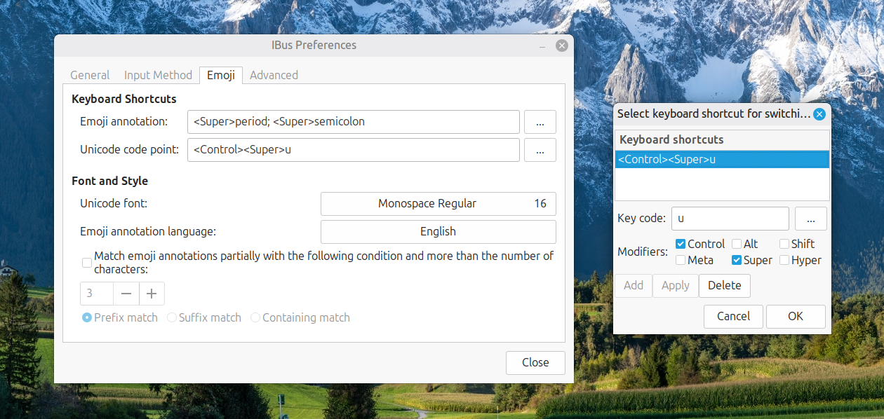
Now, I had CTRL + SUPER + U instead of CTRL + SHIFT + U. This meant that the CTRL + SHIFT + U in Enterprise Guide worked exactly as I expected it to do. A baffling situation had been resolved to leave me working without intrusion.
Modernising SAS: The 4GL Apps and SASjs Ecosystem
Custom interfaces to the world's most powerful analytics platform are no longer a niche concern. In many organisations, SAS remains central to reporting, modelling and operational decision-making, yet the way users interact with that capability can vary widely. Some teams still rely on desktop applications, batch processes, shared drives and manual interventions, while others are moving towards web-based interfaces, stronger governance and a more modern development workflow. The material at sasapps.io points to an ecosystem built around precisely that transition, blending long-standing SAS expertise with open-source tooling and documented delivery methods.
The Company Behind the Ecosystem
At the centre of this transition is 4GL Apps. The company's positioning is straightforward: help organisations leverage their SAS investment through services, solutions and products that fit specific needs. Rather than replacing SAS, the aim is to extend it with custom interfaces and delivery approaches that are maintainable, transparent and based on standard frameworks. An emphasis on documentation appears throughout the site, suggesting that projects are intended either for handover to internal teams or for ongoing support under clearly defined packages.
That proposition matters because many SAS environments have grown over years, sometimes decades. In such settings, technical capability is rarely the issue. The challenge is more often how to expose that capability in ways that are usable, secure and sustainable. A powerful analytics platform can still be hampered by awkward user journeys, brittle desktop tooling or resource-heavy support arrangements, and the 4GL Apps model tries to address those practical concerns without discarding existing SAS infrastructure.
Services
The service offering gives a useful sense of how this approach is organised. One strand is SAS App Delivery, framed not merely as building applications, but also as building tools that make SAS app development faster. That detail points to an emphasis on repeatability rather than one-off implementation. Another strand is SAS App Support, aimed at organisations with existing SAS-powered applications but insufficient internal resource to keep them running. Fixed-price plans are offered to keep those interfaces active, which implies an attempt to make operational costs more predictable. A third service area is SASjs Enhancement, where new features can be added to SASjs at a discounted rate to support particular use cases.
Solutions
These services sit alongside a broader set of solutions. One is the creation of SAS-powered HTML5 applications, described as bespoke builds tailored to specific workflow and reporting requirements, using fully open-source tools, standard frameworks and full documentation. Clients are given a practical choice: maintain the application in-house or use a transparent support package. Another solution addresses end-user computing risk through data capture and control. Here, the approach enables business users to self-load VBA-driven Excel reporting tools into a preferred database while applying data quality checks at source, a four-eyes (or more) approval step at each stage and full audit traceability back to the original EUC artefact. A further solution is the modernisation of legacy AF/SCL desktop applications, with direct migration to SAS 9 or Viya in order to improve user experience, security and scalability while moving to a modern SAS stack supported by open-source technology.
That last area reveals a theme running through the whole ecosystem: modernisation does not necessarily mean abandoning what exists. In many SAS estates, AF/SCL applications remain deeply embedded in business processes, and replacing them outright can be costly and risky, especially when they encode years of operational logic. A migration path that preserves business function while improving maintainability and interface design will naturally appeal to teams that need progress without disruption.
Products
The product range fills out the picture further. Data Controller for SAS enables business users to make controlled changes to data in SAS. The SASjs Framework is a collection of open-source tools to accelerate SAS DevOps and the development of SAS-powered web applications. There is also an AF/SCL Kit, migration tooling for the rapid modernisation of monolithic AF/SCL applications. Together, these products form a stack covering interface delivery, governed data change and development workflow, and they suggest that the company's work is not limited to consultancy but includes reusable software assets with their own documentation and source code.
Data Controller: Governance and Audit
Data Controller receives the richest functional description in the ecosystem's documentation. It is intended for business owners in regulatory reporting environments and, more broadly, for any enterprise that needs to perform manual data uploads with validation, approval, security and control. The rationale is rooted in familiar SAS working practices. Users may place files on network drives for batch loading, update data directly using SAS code, open a dataset in Enterprise Guide and change a value, or ask a database administrator to run a script update. According to the product's own documentation, those approaches are less than ideal: every new piece of data may require a new programme, end users may need to have `modify` access to sensitive data locations, datasets can become locked, and change requests can slow the process.
Data Controller is presented as a response to those weaknesses. The goal is described as focusing on great user experience and auditor satisfaction, while saving years of development and testing compared with a custom-built alternative. It is a SAS-powered web application with real-time capabilities, where intraday concurrent updates are managed using a lock table and queuing mechanism. Updates are aborted if another user has changed the table since the approval difference was generated, which helps preserve consistency in multi-user environments. Authentication and authorisation rely on the existing SASLogon framework, and end users do not require direct access to the target tables.
The governance model is equally central. All data changes require one or more approvals before a table is updated, and the approver sees only the changes that will be applied to the target, including new, deleted and changed rows. The system supports loading tables of different types through SAS libname engines, with support for retained keys, SCD2 loads, bitemporal data and composite primary keys. Full audit history is a prominent feature: users can track every change to data, including who made it, when it was made, why it was made and what the actual change was, all accessible through a History page.
A particularly notable feature is that onboarding new tables requires zero code. Adding a table is a matter of configuration performed within the tool itself, without the need to define column types or lengths manually, as these are determined dynamically at runtime. Workflow extensibility is built in through configurable hook scripts that execute before and after each action, with examples such as running a data quality check after uploading a mapping table or running a model after changing a parameter. Taken together, those features position Data Controller less as a narrow upload utility and more as a governed operational layer for business-managed data change.
The application was designed to work on multiple devices and different screen types, combined with SAS scalability and security to provide flexibility and location independence when managing data. This suggests it is intended for practical day-to-day use by business teams rather than solely by technical specialists at a desktop workstation.
SASjs: DevOps for SAS
Underpinning much of the ecosystem is SASjs, described on its GitHub organisation page as "DevOps for SAS." It is designed to accelerate the development and deployment of solutions on all flavours of SAS, including Viya, EBI and Base. Everything in SASjs is MIT open-source and free for commercial use. The framework also explicitly underpins Data Controller for SAS, which connects the product and framework strands of the wider ecosystem. The GitHub organisation page notes that the SASjs project and its repositories are not affiliated with SAS Institute.
The resources page at sasjs.io lists the key GitHub repositories: the Macro Core library, the SASjs adapter for bidirectional SAS and JavaScript communication, the SASjs CLI, a minimal seed application and seed applications for React and Angular. Documentation sites cover the adapter, CLI, Macro Core library, SASjs Server and Data Controller. Useful external links from the same resources page include guides to building and deploying web applications with the SASjs CLI, scaffolding SAS projects with NPM and SASjs, extending Angular web applications on Viya and building a vanilla JavaScript application on SAS 9 or Viya. There is also mention of a Viya log parser, training resources, guides, FAQs and a glossary, pointing to an effort to support both implementation and adoption.
The SASjs CLI
The command-line tooling, documented at cli.sasjs.io, gives a clearer view of how SASjs approaches DevOps. The CLI is described as a Swiss-army knife with a flexible set of options and utilities for DevOps on SAS Viya, SAS 9 EBI and SASjs Server. Its core functions include creating a SAS Git repository in an opinionated way, compiling each service with all dependent macros, macro variables and pre- or post-code, building the master SAS deployment, deploying through local scripts and remote SAS programmes, running unit tests with coverage and generating a Doxygen documentation site with data lineage, homepage and project logo from the configuration file. There is also a feature for deploying a frontend as a streaming application, bypassing the need to access the SAS web server directly.
The full command set covers the project lifecycle. The CLI can add and authenticate targets, compile and build projects, deploy them to a SAS server location, generate documentation and manage contexts, folders and files. It can execute jobs, run arbitrary SAS code from the terminal, deploy a service pack and generate a snippets file for macro autocompletion in VS Code. It can also lint SAS code to identify common problems and run unit tests while collecting results in JSON or CSV format, together with logs. In effect, this brings SAS development considerably closer to the workflows commonly seen in mainstream software engineering, which may be especially valuable in organisations trying to standardise delivery practices across mixed technology estates.
Presentations and the Wider SAS Community
The slides.sasjs.io collection adds another dimension by showing that these ideas have been presented in conference and user group settings. Available decks cover DevOps for MSUG, SUGG and WUSS, SASjs for application development, SASjs Server, AF and AF/SCL modernisation, SASjs for PHUSE, testing and a legacy SAS apps presentation for FANS in January 2023. While slide decks alone do not prove adoption or outcomes, they do show a sustained effort to communicate methods and patterns to the broader SAS community, consistent with the open documentation and MIT licensing found throughout the ecosystem.
Building a Modern Layer Around an Established Platform
The most useful way to understand this ecosystem is not as a single product but as a layered approach. At one level, there are services for building and supporting applications. At another, there are packaged tools such as Data Controller and the AF/SCL Kit. Underneath both sits SASjs, providing open-source components and delivery practices intended to make SAS development more structured and scalable. The combination of bespoke SAS-powered HTML5 applications, governed data update tooling, AF/SCL migration support and open-source DevOps utilities points to a coherent effort to modernise how SAS is delivered and used, without severing ties to established platforms. SAS remains the analytical engine, but the interfaces, workflows and operational controls around it are updated to reflect current expectations in web application design, governance and DevOps practice.
Launching SAS Analytics Pro on Viya with automated Docker image clean-up
For my freelancing, I have a licensed version of SAS Analytics Pro running in a Docker container on my main Linux workstation. Every time there is a new release, a new Docker is made available, which means that a few of them could accumulate on your system. Aside from taking up disk space that could have other uses, it also makes it tricky to automate the startup of the associate Docker container. Avoiding this means pruning the Docker images available on the system, something that also needs automation.
To make things clearer, let me work through the launch script that I use; this is called by the script that checks for and then downloads any new image that is available, should that be needed. First up is the shebang, and this uses the -e switch to exit the script in the event of there being an error. That puts a stop to any potentially destructive outcomes from later commands being executed afterwards and without having the input that they need.
#!/bin/bash -e
Next comes the command to shut down the existing container. Should a new image get instated, this would lock up the old one, preventing its removal. Also, doing the rest of the steps with an already running container will result in errors anyway.
if docker container ls -a --format '{{.Names}}' | grep -q '^sas-analytics-pro$'; then
    docker container stop sas-analytics-pro
fi
After that, the step to find the latest image is performed. Once, I did this by looping through the ages by days, weeks and months, hardly an elegant or robust approach. What follows is something all the more effective.
# Find latest SAS Analytics Pro image
IMAGE=$(docker image ls --format '{{.Repository}}:{{.Tag}} {{.CreatedAt}}' \
    | grep 'sas-analytics-pro' \
    | sort -k2,3r \
    | head -n 1 \
    | awk '{print $1}')

echo "Chosen image: $IMAGE"
Since there is quite a lot happening above, let us unpack the actions. The first part lists all Docker images, formatting each line to show the image name (repository:tag) followed by its creation timestamp: docker image ls --format '{{.Repository}}:{{.Tag}} {{.CreatedAt}}'. The next piece picks out all the images that are for SAS Analytics Pro: grep 'sas-analytics-pro'. The crucial step, sort -k2,3r, comes next and this sorts the results by the second and third fields (the creation date and time) in reverse order, so the newest images appear first. With that done, it is time to pick out the most recent image using head -n 1. To pick out the image name, you need awk '{print $1}. This wrapped within IMAGE=$(...) to assign the result to a variable that is printed to the console using an echo statement.
With the image selected, you can then spin up the container once you specify the other parameters to use and allow some sleep time afterwards before proceeding to the clean-up steps:
run_args="
-e SASLOCKDOWN=0
--name=sas-analytics-pro
--rm
--detach
--hostname sas-analytics-pro
--env RUN_MODE=developer
--env SASLICENSEFILE=[Path to SAS licence file]
--publish 8080:80
--volume ${PWD}/sasinside:/sasinside
--volume ${PWD}/sasdemo:/data2
--volume [location of SAS files on the system]:/data
--cap-add AUDIT_WRITE
--cap-add SYS_ADMIN
--publish 8222:22
"

if ! docker run -u root ${run_args} "$IMAGE" "$@" > /dev/null 2>&1; then
    echo "Failed to run the image."
    exit 1
fi

sleep 5
With the new container in action, the subsequent step is to find the older images and delete those. Again, the docker image command is invoked, with its output fed to a selection command for SAS Analytics Pro images. Once the current image has been removed from the listing by the grep -v command, the list of images to be deleted is assigned to the IMAGES_TO_REMOVE variable.
IMAGES_TO_REMOVE=$(docker image ls --format '{{.Repository}}:{{.Tag}}' \
    | grep 'sas-analytics-pro' \
    | grep -v "^$IMAGE$")

echo "Will remove older images:"
echo "$IMAGES_TO_REMOVE"
After that has happened, iterating through the list of images using a for loop will remove them one at a time using the docker image rm command:
for OLD in $IMAGES_TO_REMOVE; do
    echo "Removing $OLD"
    docker image rm "$OLD" || echo "Could not remove $OLD"
done
All this concludes the operation of spinning up a new SAS Analytics Pro Docker container while also removing any superseded Docker images. One last step is to capture the password to use for logging into the SAS Studio interface that is available at localhost:8080 or whatever address and port is being used to serve the application:
docker logs sas-analytics-pro 2>&1 | grep "Password=" > pw.txtFolding updating and housekeeping into the same activity as spinning up the Docker container means that I need not think of doing anything else. The time taken by the other activities repay the effort by always having the latest version running in a tidy environment. That just saves having to remember to do all of this, which is what is needed without automation.
Using the LIKE operator in PROC SQL WHERE clauses in SAS
Recently, I was working in SAS and decided to trying picking out datasets and variables from its dictionary tables, eventually picking out the maximum length of a variable type for assigning the length of a new variable. This could have been done using a long-established technique:
proc sql;
    select distinct memname into :dsns separated by '#'
        from dictionary.tables
            where lowcase(libname) = 'work'
            and index(lowcase(memname), "r_") = 1
            and index(lowcase(memname), "visit") = 0;
quit;
The result is that it creates a macro variable containing a delimited list of work datasets with names beginning with r_ and not containing the string visit. As well as using the index function to find the placing of one string within another, I have seen the count function used for similar purposes, albeit without the placement specificity. Since the =: operator which looks for a search string at the start of a larger is not something that works in SQL (data step is more than fine), you cannot do something like this:
proc print data = sashelp.vmember noobs;
    where lowcase(libname) = 'work'
    and lowcase(memname) =: "r_";
run;
While the contains operator works similarly to the count function when it comes to search text positioning, yet another option is the like operator, and that is shown in the example below:
proc sql;
    select distinct memname into :dsns separated by '#'
        from dictionary.tables
            where lowcase(libname) = 'work'
            and lowcase(memname) like 'r\_%' escape '\'
            and lowcase(memname) not like '%visit%';
quit;
Here, % and _ are placeholder characters, with the first matching zero or more characters and the second matching one character. Thus, the underscore in r_ needs escaping to look for that pattern (otherwise, it will look for the letter r at the start of a string and a single character after it) and a backslash character (\) will cover that duty. To ensure that it does what you want, adding escape '\' after the expression tells SAS what is happening.
Another thing to watch is that the percent (%) character needs a form escaping from the SAS Macro language processor, and placing the search term in single quotes attends to that. That means that %visit% does not cause any errors when you are looking for visit within a dataset name and using negation (the not operator) to exclude that possibility from the search results. However, using _%visit% might be a better pattern for finding visit at the end of a name, though.
Should you wish to play around with the above to see what happens for your own learning, try using something like this to give you a few test datasets:
data r_test r_visit visit;
    set sashelp.class;
run;
Otherwise, feel free to add your own test cases to cement the ideas even further. All too often, we look up something, deploy it and then forget about, especially when AI is involved. Nevertheless, the fastest way to write code can be to use what is embedded in your memory.
WARNING: Unsupported device 'SVG' for RTF destination. Using default device 'EMF'.
When running SAS programs to create some outputs, I met with the above message because I was sending output to an RTF file and these do not support SVG files. This must be a system default because there was nothing in the programs that should trigger the warning. Getting rid of the message uses one of two approaches:
goptions device=emf;
ods graphics / outputfmt=emf;
The first applies to legacy code generating graphics using SAS/GRAPH procedures, while the second is for the more modern ODS graphics procedures like SGPLOT. While the first one may work in all cases, that cannot be assumed without further testing.
There was another curiosity in this: the system setup should have taken care of things to stop the warning from appearing in the log. However, these were programs created from SAS logs to capture all code generated by any SAS macros that were called for regulatory submission purposes. Thus, they were self-contained and missed off the environment setup code, which is how I came to see what I did.
Platform-independent file deletion in SAS programming
There are times when you need to delete a file from within a SAS program that is not one of its inbuilt types, such as datasets or catalogues. Many choose to use X commands or the SYSTASK facility, even if these issue operating system-specific commands that obstruct portability. Also, it should be recalled that system administrators can make these unavailable to users as well. Thus, it is better to use methods that are provided within SAS itself.
The first step is to define a file reference pointing to the file that you need to delete:
filename myfile '<full path of file to be removed>';
With that accomplished, you can move on to deleting the file in a null data step, one where no output file is generated. The FDELETE function does that in the code below using the MYFILE file reference declared already. That step issues a return code used in the provision of feedback to the user, with 0 indicated success and non-zero values indicating failure.
data _null_;
  rc = fdelete('myfile');
  if rc = 0 then put 'File deleted successfully.';
  else put 'Error deleting file. RC=' rc;
run;
With the above out of the way, you then can clear the file reference to tidy up things afterwards:
filename myfile clear;
Some may consider that SAS programs are single use items that may not be moved from one system to another. However, I have been involved in several of these, particularly between Windows, UNIX and Linux, so I know the value of keeping things streamlined and some SAS programs are multi-use anyway. Anything that cuts down on workload when there is much else to do cannot be discounted.