TOPIC: MICROSOFT EXCEL
Some R functions for working with dates, strings and data frames
Working with data in R often comes down to a handful of recurring tasks: combining text, converting dates and times, reshaping tables and creating summaries that are easier to interpret. This article brings together several strands of base R and tidyverse-style practice, with a particular focus on string handling, date parsing, subsetting and simple time series smoothing. Taken together, these functions form part of the everyday toolkit for data cleaning and analysis, especially when imported data arrive in inconsistent formats.
String Building
At the simplest end of this toolkit is paste(), a base R function for concatenating character vectors. Its purpose is straightforward: it converts one or more R objects to character vectors and joins them together, separating terms with the string supplied in sep, which defaults to a space. If the inputs are vectors, concatenation happens term by term, so paste("A", 1:6, sep = "") yields "A1" through "A6", while paste(1:12) behaves much like as.character(1:12). There is also a collapse argument, which takes the resulting vector and combines its elements into a single string separated by the chosen delimiter, making paste() useful both for constructing values row by row and for creating one final display string from many parts.
That basic string-building role becomes more important when dates and times are involved because imported date-time data often arrive as text split across multiple columns. A common example is having one column for a date and another for a time, then joining them with paste(dates, times) before parsing the result. In that sense, the paste() function often acts as a bridge between messy raw input and structured date-time objects. It is simple, but it appears repeatedly in data preparation pipelines.
Date-Time Conversion
For date-time conversion, base R provides strptime(), strftime() and format() methods for POSIXlt and POSIXct objects. These functions convert between character representations and R date-time classes, and they are central to understanding how R reads and prints times. strptime() takes character input and converts it to an object of class "POSIXlt", while strftime() and format() move in the other direction, turning date-time objects into character strings. The as.character() method for "POSIXt" classes fits into the same family, and the essential idea is that the date-time value and its textual representation are separate things, with the format string defining how R should interpret or display that representation.
Format strings rely on conversion specifications introduced with %, and many of these are standard across systems. %Y means a four-digit year with century, %y means a two-digit year, %m is a month, %d is the day of a month and %H:%M:%S captures hours, minutes and seconds in 24-hour time. %F is equivalent to %Y-%m-%d, which is the ISO 8601 date format. %b and %B represent abbreviated and complete month names, while %a and %A do the same for weekdays. Locale matters here because month names, weekday names, AM/PM indicators and some separators depend on the LC_TIME locale, meaning a date string like "1jan1960" may parse correctly in one locale and return NA in another unless the locale is set appropriately.
R's defaults generally follow ISO 8601 rules, so dates print as "2001-02-28" and times as "14:01:02", though R inserts a space between date and time by default. Several details matter in practice. strptime() processes input strings only as far as needed for the specified format, so trailing characters are ignored. Unspecified hours, minutes and seconds default to zero, and if no year, month or day is supplied then the current values are assumed, though if a month is given, the day must also be valid for that month. Invalid calendar dates such as "2010-02-30 08:00" produce results whose components are all NA.
Time Zones and Daylight Saving
Time zones add another layer of complexity. The tz argument specifies the time zone to use for conversion, with "" meaning the current time zone and "GMT" meaning UTC. Invalid values are often treated as UTC, though behaviour can be system-specific. The usetz argument controls whether a time zone abbreviation is appended to output, which is generally more reliable than %Z. %z represents a signed UTC offset such as -0800, and R supports it for input on all platforms. Even so, time zones can be awkward because daylight saving transitions create times that do not occur at all, or occur twice, and strptime() itself does not validate those cases, though conversion through as.POSIXct may do so.
Two-Digit Years
Two-digit years are a notable source of confusion for analysts working with historical data. As described in the R date formats guide on R-bloggers, %y maps values 00 to 68 to the years 2000 to 2068 and 69 to 99 to 1969 to 1999, following the POSIX standard. A value such as "08/17/20" may therefore be interpreted as 2020 when the intended year is 1920. One practical workaround is to identify any parsed dates lying in the future and then rebuild them with a 19 prefix using format() and ifelse(). This approach is explicit and practical, though it depends on the assumptions of the data at hand.
Plain Dates
For plain dates, rather than full date-times, as.Date() is usually the entry point. Character dates can be imported by specifying the current format, such as %m/%d/%y for "05/27/84" or %B %d %Y for "May 27 1984". If no format is supplied, as.Date() first tries %Y-%m-%d and then %Y/%m/%d. Numeric dates are common when data come from Excel, and here the crucial issue is the origin date: Windows Excel uses an origin of "1899-12-30" for dates after 1900 because Excel incorrectly treated 1900 as a leap year (an error originally copied from Lotus 1-2-3 for compatibility), while Mac Excel traditionally uses "1904-01-01". Once the correct origin is supplied, as.Date() converts the serial numbers into standard R dates.
After import, format() can display dates in other ways without changing their underlying class. For example, format(betterDates, "%a %b %d") might yield values like "Sun May 27" and "Thu Jul 07". This distinction between storage and display is important because once R recognises values as dates, they can participate in date-aware operations such as mean(), min() and max(), and a vector of dates can have a meaningful mean date with the minimum and maximum identifying the earliest and latest observations.
Extracting Columns and Manipulating Lists
These ideas about correct types and structure carry over into table manipulation. A data frame column often needs to be extracted as a vector before further processing, and there are several standard ways to do this, as covered in this guide from Statistics Globe. In base R, the $ operator gives a direct route, as in data$x1. Subsetting with data[, "x1"] yields the same result for a single column, and in the tidyverse, dplyr::pull(data, x1) serves the same purpose. All three approaches convert a column of a data frame into a standalone vector, and each is useful depending on the surrounding code style.
List manipulation has similar patterns, detailed in this Statistics Globe tutorial on removing list elements. Removing elements from a list can be done by position with negative indexing, as in my_list[-2], or by assigning NULL to the relevant component, for example my_list_2[2] <- NULL. If names are more meaningful than positions, then subsetting with names(my_list) != "b" or names(my_list) %in% "b" == FALSE removes the named element instead. The same logic extends to multiple elements, whether by positions such as -c(2, 3) or names such as %in% c("b", "c") == FALSE. These are simple techniques, but they matter because lists are a common structure in R, especially when working with nested results.
Subsetting, Renaming and Reordering Data Frames
Data frames themselves can be subset in several ways, and the choice often depends on readability, as the five-method overview on R-bloggers demonstrates clearly. The bracket form example[x, y] remains the foundation, whether selecting rows and columns directly or omitting unwanted ones with negative indices. More expressive alternatives include which() together with %in%, the base subset() function and tidyverse verbs like filter() and select(). The point is not that one method is universally best, but that R offers both low-level precision and higher-level readability, depending on the task.
Column names and column order also need regular attention. Renaming can be done with dplyr::rename(), as explained in this lesson from Datanovia, for instance changing Sepal.Length to sepal_length and Sepal.Width to sepal_width. In base R, the same effect comes from modifying names() or colnames(), either by matching specific names or by position. Reordering columns is just as direct, with a data frame rearranged by column indices such as my_data[, c(5, 4, 1, 2, 3)] or by an explicit character vector of names, as the STHDA guide on reordering columns illustrates. Both approaches are useful when preparing data for presentation or for functions that expect variables in a certain order.
Sorting and Cumulative Calculations
Sorting and cumulative calculations fit naturally into this same preparatory workflow. To sort a data frame in base R, the DataCamp sorting reference demonstrates that order() is the key function: mtcars[order(mpg), ] sorts ascending by mpg, while mtcars[order(mpg, -cyl), ] sorts by mpg ascending and cyl descending. For cumulative totals, cumsum() provides a running sum, as in calculating cumulative air miles from the airmiles dataset, an example covered in the Data Cornering guide to cumulative calculations. Within grouped data, dplyr::group_by() and mutate() can apply cumsum() separately to each group, and a related idea is cumulative count, which can be built by summing a column of ones within groups, or with data.table::rowid() to create a group index.
Time Series Smoothing
Time series smoothing introduces one further pattern: replacing noisy raw values with moving averages. As the Storybench rolling averages guide explains, the zoo::rollmean() function calculates rolling means over a window of width k, and examples using 3, 5, 7, 15 and 21-day windows on pandemic deaths and confirmed cases by state demonstrate the approach clearly. After arranging and grouping by state, mutate() adds variables such as death_03da, death_05da and death_07da. Because rollmean() is centred by default, the resulting values are symmetrical around the observation of interest and produce NA values at the start and end where there are not enough surrounding observations, which is why odd values of k are usually preferred as they make the smoothing window balanced.
The arithmetic is uncomplicated, but the interpretation is useful. A 3-day moving average for a given date is the mean of that day, the previous day and the following day, while a 7-day moving average uses three observations on either side. As the window widens, the line becomes smoother, but more short-term variation is lost. This trade-off is visible when comparing 3-day and 21-day averages: a shorter average tracks recent changes more closely, while a longer one suppresses noise and makes broader trends stand out. If a trailing rather than centred calculation is needed, rollmeanr() shifts the window to the right-hand end.
The same grouped workflow can be used to derive new daily values before smoothing. In the pandemic example, daily new confirmed cases are calculated from cumulative confirmed counts using dplyr::lag(), with each day's new cases equal to the current cumulative total minus the previous day's total. Grouping by state and date, summing confirmed counts and then subtracting the lagged value produces new_confirmed_cases, which can then be smoothed with rollmean() in the same way as deaths. Once these measures are available, reshaping with pivot_longer() allows raw values and rolling averages to be plotted together in ggplot2, making it easier to compare volatility against trend.
How These R Data Manipulation Techniques Fit Together
What links all of these techniques is not just that they are common in R, but that they solve the mundane, essential problems of analysis. Data arrive as text when they should be dates, as cumulative counts when daily changes are needed, as broad tables when only a few columns matter, or as inconsistent names that get in the way of clear code. Functions such as paste(), strptime(), as.Date(), order(), cumsum(), rollmean(), rename(), select() and simple bracket subsetting are therefore less like isolated tricks and more like pieces of a coherent working practice. Knowing how they fit together makes it easier to move from raw input to reliable analysis, with fewer surprises along the way.
Practical Excel skills for dates, locked files and text splitting
Excel has a reputation for simplicity that does not always survive contact with real working life. Project schedules need to respect weekends and public holidays, files arrive locked at precisely the moment edits are most urgent, and data lands in cells formatted in ways that resist immediate analysis. Three everyday tasks illustrate this gap well: calculating future or past dates that exclude non-working days, removing or working around read-only restrictions when genuine edits are required, and splitting text strings cleanly at the first or Nth delimiter. The guidance below draws on established Excel features, keeping the emphasis firmly on what works in practice.
Working with Business Calendars
The WORKDAY Function
Working with dates that observe a business calendar is a frequent requirement in scheduling, logistics and reporting. Excel's WORKDAY function is designed for this purpose and returns a date that is a given number of working days from a start date, excluding Saturdays and Sundays by default. At its simplest, a formula such as =WORKDAY(A1,5) moves forward five working days from the date in A1. The function can also respect a list of holidays so that results avoid specific non-working dates as well as weekends, as in =WORKDAY(A1,5,C1:C3), which skips any matching dates in C1:C3 when calculating the result.
A concrete example shows how this behaves with a real date. Using named ranges for readability, with start referring to cell B5, days to B8, and holidays to B11:B13, the formula =WORKDAY(start,days) returns the next working day five days after 23rd December 2024. With weekends excluded, but no holidays provided, the result is Monday 30th December 2024. When holidays are supplied with =WORKDAY(start,days,holidays), the function also avoids the listed dates in B11:B13 and produces Thursday 2nd January 2025. In all cases, the weekend definition is Saturday and Sunday, and the holidays must be stored as valid Excel dates to be recognised correctly.
Visualising the Path to the Result
It often helps to see the individual dates that WORKDAY steps through when reaching its answer. A compact way to achieve this is to generate a short run of consecutive dates from the start date and display them alongside abbreviated day names. Using =SEQUENCE(13,1,start) in cell D5 creates thirteen dates beginning with the date held in the named range start because Excel dates are serial numbers that increment by one per day. Formatting these cells with the custom number format ddd, dd-mmm-yy shows an abbreviated weekday alongside the date, making it straightforward to spot weekends at a glance.
Conditional formatting can then shade non-working days directly within this generated block. Because WORKDAY does not evaluate a date when zero is supplied for the argument called days, a small workaround helps determine whether a given date is itself a working day. In column D, a rule based on the formula =WORKDAY(D5-1,1)<>D5 asks WORKDAY for the next working day after the previous day; if the answer does not equal the date in D5, then D5 is not a working day and can be shaded grey. A similar rule for column E, =WORKDAY(E5-1,1,holidays)<>E5, incorporates the named holiday range and produces additional shading where dates overlap with the supplied holiday list as well as weekends.
Highlighting calculated end dates ties the visualisation together. If the main results appear in G5 and G6, cells in column D can be highlighted when equal to $G$5 using a rule such as =D5=$G$5, and cells in column E can be highlighted when equal to $G$6 using =E5=$G$6. If preferred, the formatting rules can be defined without relying on G5 and G6 by embedding the WORKDAY calls directly in the comparisons, as in =D5=WORKDAY(start,days) and =E5=WORKDAY(start,days,holidays). In either arrangement, there are four conditional formatting rules in play across the grid: two to shade non-working days and two to pick out the final dates.
Handling Non-Standard Working Weeks
Work patterns do not always match the standard five-day week. Where a schedule follows a different rhythm, such as a four-day or six-day working week, switching to the WORKDAY.INTL function is the appropriate step. It follows the same principle as WORKDAY, returning a date a set number of business days from a start date while optionally excluding holidays, but it accepts a custom definition of which weekdays count as working days. This flexibility allows organisations that operate alternative rosters to generate accurate due dates without resorting to manual adjustments or complex helper columns.
Managing Read-Only Excel Files
There are several reasons why a workbook might be set to read-only: preventing accidental erasure of data, or ensuring a file remains unchanged as it passes between parties. Each form of protection serves a different purpose and has a distinct method for disabling it. ExcelRibbon.Tips.Net is a useful ongoing reference for these and many other workbook and security scenarios across Excel 2007 and later versions.
Read-Only Recommended
The lightest touch is the Read-Only Recommended setting. When a workbook carries this flag, Excel prompts on opening with a dialogue asking whether to open it as read-only. This method applies across all versions of Microsoft Excel from 2003 through to current releases. To remove the recommendation, open the workbook, use File > Save As and choose Browse to open the Save As window, then select Tools in the lower right of the dialogue, pick General Options, clear the Read-Only Recommended checkbox and click OK before saving. The next time the file opens, the prompt does not appear.
Marked as Final
A firmer signal is applied when a workbook is Marked as Final. In this state, commands, typing and proofing marks are all disabled, and Excel displays a Marked as Final notification bar at the top of the worksheet. To turn this off when editing is required, click Edit Anyway on the notification bar. This removes the read-only state for the current copy and allows modifications to proceed. The flag is more about signalling completion than enforcing security, so the application provides a clear override directly within the interface.
Password to Modify
Password protection introduces a stronger barrier. When a workbook has a Password to Modify set, a dialogue appears on opening that invites the password or offers the option to open the file as read-only; without the password, the file cannot be modified directly. A pragmatic path when only a working copy is needed is to open the original in read-only mode, then use File > Save As with Browse, select Tools > General Options, clear the Password to Modify field and confirm with OK before saving under a new name. Opening the newly saved file allows edits because it no longer carries a modification password. Using a third-party utility to crack a password on someone else's file is inadvisable and potentially inappropriate, so the better route is to request an editable version from whoever sent the document.
Operating System-Level Restrictions on a Mac
Occasionally, the read-only state is imposed not by Excel but by the operating system, where the file has been locked so that only the owner can edit it. On a Mac, the fix is made outside Excel: locate the file in Finder, right-click it and choose Get Info, then clear the Locked checkbox before reopening the file in Excel. If the issue is one of permissions rather than a simple lock, the Get Info window also contains a Sharing and Permissions section at the bottom. This lists each user alongside a drop-down privilege set to either Read Only or Read and Write, and the file owner can adjust these entries to grant editing access to the relevant users.
Operating System-Level Restrictions on a PC
On a PC, the equivalent controls are found in File Explorer. Right-clicking the workbook and choosing Properties opens the General tab, where unchecking the Read-Only attribute and clicking OK is often sufficient to restore full access. If the restriction stems from security permissions rather than the file attribute, the Security tab lists the groups and usernames that have access along with their permission levels. Clicking Edit beneath that list allows the file owner to adjust access for individual entries, including granting the ability to modify the file where that is justified.
Splitting Text in Excel
LEFT, MID and RIGHT
Reshaping text is another everyday requirement in Excel, and the LEFT, MID and RIGHT functions provide predictable building blocks. LEFT extracts a specified number of characters from the start of a string, MID extracts from a given position in the middle, and RIGHT extracts from the end. For instance, =LEFT("test string",2) returns te, =MID("test string",6,3) returns str, and =RIGHT("test string",2) returns ng. When exact character counts are known in advance these functions can be applied directly, but real data often arrives with variable-length segments separated by spaces or other delimiters, so the position of the delimiter must first be discovered before extraction can take place.
Splitting at the First Delimiter
To split at the first occurrence of a delimiter such as a space, combining these extraction functions with FIND or SEARCH is effective. Both functions return the position of a substring within a string, with the key distinction that FIND is case-sensitive while SEARCH is not. Suppose cell A1 contains test string. To return everything to the left of the first space, use =LEFT(A1,FIND(" ",A1)-1). Here FIND returns 5 as the position of the space, subtracting 1 yields 4, and LEFT uses that figure to return test. To return the text to the right of the first space, the formula subtracts the space position from the total string length: =RIGHT(A1,LEN(A1)-FIND(" ",A1)). In this example, LEN(A1) is 11 and the FIND result is 5, so the expression evaluates to 6 and RIGHT returns string. The pattern generalises to other delimiters by replacing the space character with the required alternative.
Locating the Nth Delimiter
Locating the Nth occurrence of a delimiter takes an extra step because FIND and SEARCH identify only the first match after a given starting point. A common technique relies on SUBSTITUTE to mark the Nth occurrence with a unique character that does not appear elsewhere in the text, then uses FIND to locate it. Consider An example text string in A1 and a requirement to return everything up to the third space. Substituting the third space with a vertical bar creates a dependable marker: =SUBSTITUTE(A1," ","|",3) produces An example text|string. Finding the bar with =FIND("|",SUBSTITUTE(A1," ","|",3)) returns 16, the position of the marker. LEFT can then extract the part before that position by subtracting one: =LEFT(A1,FIND("|",SUBSTITUTE(A1," ","|",3))-1), which returns An example text. Combining the steps in this way makes the formula self-contained and avoids the need for helper cells.
These text approaches extend naturally to extracting the segment after the Nth delimiter by using MID or RIGHT, with similar position logic. Replacing LEFT with MID and adjusting the start index to the marker position plus one retrieves the portion that follows. The same idea works with second or fourth occurrences by changing the instance number inside SUBSTITUTE. When working with data sets that include inconsistent spacing or punctuation, it is worth verifying that the chosen marker character does not already appear in the source text, since the method depends on its uniqueness within each processed string.
Bringing These Techniques Together in Your Excel Workflows
These three strands combine to form a toolkit that handles a surprising range of everyday scenarios. WORKDAY and WORKDAY.INTL anchor date calculations to real-world calendars so that estimates and commitments respect weekends and public holidays, while the SEQUENCE-based visualisation grid can help colleagues understand how an end date is reached rather than simply accepting a single cell value. Managing read-only states allows teams to balance protection with flexibility, with the key being to identify which type of restriction applies before attempting to remove it. LEFT, MID and RIGHT, combined with FIND and SUBSTITUTE, turn messy text into consistent fields ready for further analysis.
Adding line breaks in Excel in a Citrix Windows session on a Mac
Today, I tried connecting to a client system using my Mac Mini. Everything went well, aside perhaps from some resizing, apart from something more crucial: adding a line break in a cell in an Excel spreadsheet. The usual combination of ALT+ENTER was not doing the needful. Instead, I needed to use CMD+OPTION+ENTER, as it would be on a Mac keyboard. Since I use a Windows one inside, it looks like this: WIN+ALT+ENTER. It was only by looking through the options for the Citrix Workspace app that came upon this after being prompted to do so by ChatGPT, itself not supplying the fully correct information that I needed. Now, all I need to do is remember to use the correct keyboard shortcut, and I am away.
A way to survey hours of daylight for locations of interest
A few years back, I needed to get sunrise and sunset information for a location in Ireland. This was to help me plan visits to a rural location with a bus service going nearby, and I did not want to be waiting on the side of the road in the dark on my return journey. It ended up being a project that I undertook using the Julia programming language.
This had other uses too: one was the planning of trips to North America. This was how I learned that evenings in San Francisco were not as long as their counterparts in Ireland. Later, it had its uses in assessing the feasibility of seeing other parts of the Pacific Northwest during the month of August. Other matters meant that such designs never came to anything.
The Sunrise Sunset API was used to get the times for the start and end of daylight. That meant looping through the days of the year to get the information, but I needed to get the latitude and longitude information from elsewhere to fuel that process. While Google Maps has its uses with this, it is a manual and rather fiddly process. Sparing use of Nomintim's API is what helped with increasing the amount of automation and user-friendliness, especially what comes from OpenStreetMap.
Accessing using Julia's HTTP package got me the data in JSON format that I then converted into atomic vectors and tabular data. The end product is an Excel spreadsheet with all the times in UTC. A next step would be to use the solar noon information to port things to the correct timezone. It can be done manually in Excel and its kind, but some more automation would make things smoother.
Stop Excel 365 saving files to OneDrive by default
Recently, I was doing some work in Excel (while I use the 365 version, this may work with others too) when I found it offering to save a file to OneDrive by default. My preference is to keep everything local, especially given the limitations of online storage. Thus, I sought a way to do just this.

That meant going to File > Options and then to the Save tab. In there, I found the option called Save to Computer by default and activated that. The default local location can be changed too, but I left this as it was because I tend to use multiple file locations anyway. Clicking on the OK button after making the change that I wanted was enough to set the behaviour as I required, and I no longer see the prompt for online storage since then.
Adding titles and footnotes to Excel files created using SAS
Using the Excel and ExcelXP destinations in the Output Delivery System (ODS), SAS can generate reports as XLSX workbooks with one or more worksheets. Recently, I was updating a SAS Macro that created one of these and noticed that there were no footnotes. The fix was a simple: add to the options specified on the initial ODS Excel statement.
ods excel file="&outdir./&file_name..xlsx" options(embedded_titles="yes" embedded_footnotes="yes");
Notice in the code above that there are EMBEDDED_TITLES and EMBEDDED_FOOTNOTES options. Without both of these being set to YES, no titles or footnotes will appear in a given worksheet, even if they have been specified in a program using TITLE or FOOTNOTE statements. In my case, it was the EMBEDDED_FOOTNOTES option that was missing, so adding that set things to rights.
The thing applies to the ExcelXP tag set, as you will find from a code sample that SAS has shared on their website. That was what led me to the solution to what was happening in the Excel ODS destination in my case.
Solving SAS PROC IMPORT Error 8000101D when reading Excel files on entimICE
Recently, I encountered the following kind of message when reading an Excel file into SAS using PROC IMPORT:
ERROR: Error opening XLSX file -> xxx-.xlsx . It is either not an Excel spreadsheet or it is damaged. Error code=8000101D

Requested Input File Is Invalid

ERROR: Import unsuccessful. See SAS Log for details.
Naturally, thoughts arise regarding the state of the Excel file when you see a message like this, but that was not the case because the file opened successfully in Excel and looked OK to me. After searching on the web, I found that it was a file permissions issue. The actual environment that I was using at the time was entimICE, and I had forgotten to set up a link that granted read access to the file. Once that was added, the problem got resolved. In other systems, checking on file system permissions is needed, even if the message seems to suggest that you are experiencing a file integrity problem.
Shrinking title bar search box in Microsoft Office 365 applications

It might be a new development, but I only recently spotted the presence of a search box in the titles of both Microsoft Word and Microsoft Excel that I have as part of an Office 365 subscription. Though handy for searching file contents and checking on spelling and grammar, I also realised that the boxes take up quite a bit of space and decided to see if hiding them was possible.
![]()
In the event, I found that they could be shrunk from a box to an icon that expanded to pop up a box when you clicked on them. Since I did not need the box to be on view all the time, that outcome was sufficient for my designs, though it may not satisfy others who want to hide this functionality completely.
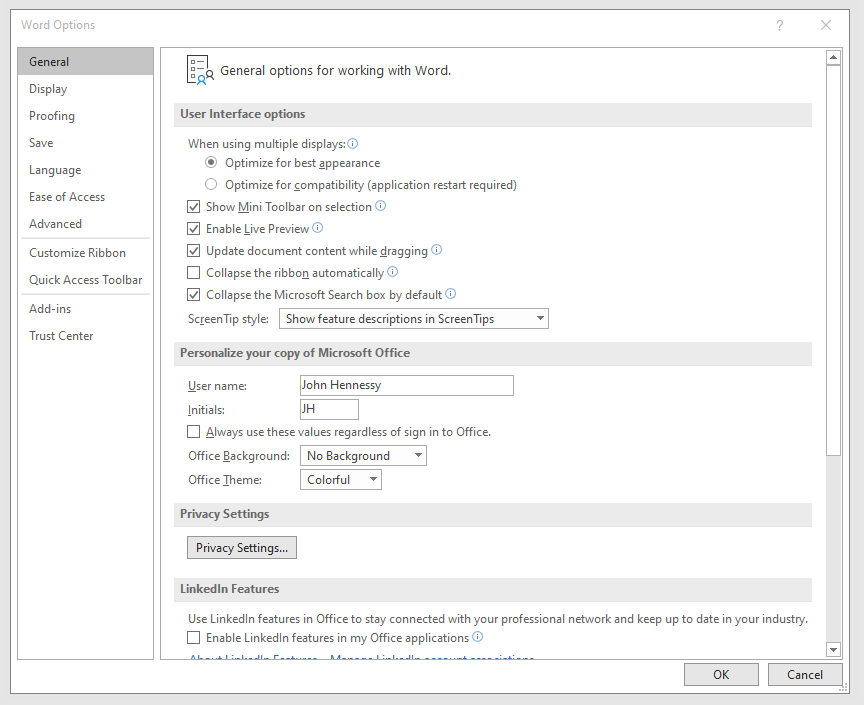
To get it, it was a matter of going to File > Options and putting a tick in the box next to the Collapse the Microsoft Search box by default entry in the General tab before clicking on the OK button. Doing that freed up some title bar space as desired, and searching is only a button press away.
A hidden cost of sharing Excel workbooks
Recently, I encountered a reason to be wary about creating shared Excel spreadsheets when one ballooned in size. It ended up growing to around 130 megabytes before I tried turning off sharing to see what happened and the size shrunk to under 200 kilobytes. From this, it would appear that the version control information was the cause of the explosion in file size.
With that in mind, I set about to looking through the settings to see if there were any that might need optimisation. While the default action is to keep thirty days of change tracking, I have this reduced to a single day in order not to be keeping too much. Quite how much you need to retain is up to you, but I will be keeping an eye on things now that I have done this.
One reason why you cannot merge cells in Excel
One handy thing that I didn't realise that you could do with Excel until the last few months was the ability to share an open workbook between users and collate any changes that are made (it seems that a form of version control is behind this). From what I have seen, Excel seems to manage changes to shared spreadsheets rather well. When you save yours, it adds updates from other users and warns if any edits collide with one another. To activate it in Excel 2003, all that needs doing is for you to go to the Share Workbook entry on the Tools and tick the appropriate checkbox in the resulting dialogue box. In 2007 and 2010, look for the Share Workbook icon in the Review tab on the ribbon to get the same dialogue box popping up.
That's not to say that it doesn't have its restrictions, though. For example, I have found that the merging of cells is made unavailable, but that can be sorted by unsharing and resharing the workbook when no one else is using it. As to why cell merger is switched off by sharing, I have a few ideas. Maybe, they couldn't make it work reliably (can happen with large software development projects like the creation of a new version of Excel) or decided that it would have consequences for other users that are too inconvenient. Either way, we cannot merge cells in shared workbooks, and that's the way that things are for now. Some may not worry about this though, since they reckon that cell merging is undesirable anyway; well, don't go doing it in any spreadsheet that is likely to be read in by another program, or you could cause trouble.